动手学深度学习v2

课程链接：https://courses.d2l.ai/zh-v2/

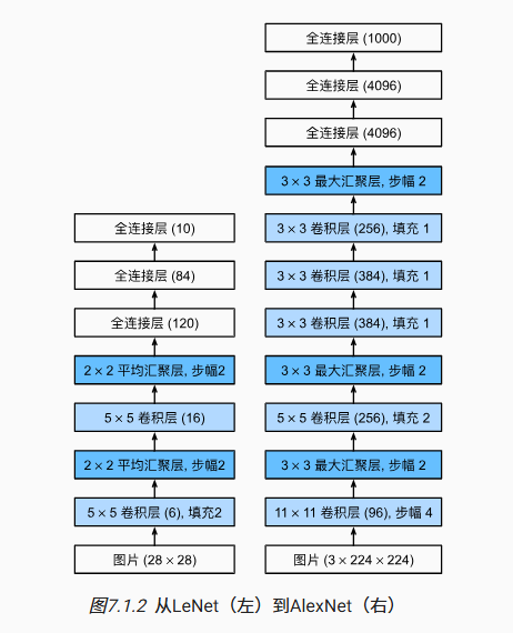
深度卷积神经网络 AlexNet

AlexNet

相比于LeNet：

更深更宽
激活函数从sigmoid变成ReLU（减缓梯度消失）
隐藏全连接层后加入了丢弃层
数据增强

代码实现

 1
 2
 3
 4
 5
 6
 7
 8
 9
10
11
12
13
14
15
16
17
18
19
20
21
22
23
24
25
26
27
28
29
30
31
32
33
34
35
36
37
38
39
40
41
42
43
44
45
46
47
48
49
50
51
52
53
54
55
56
57
58
59
60
61
62
63


import torch
from torch import nn
from d2l import torch as d2l

net = nn.Sequential(
    # 这里使用一个11*11的更大窗口来捕捉对象。
    # 同时，步幅为4，以减少输出的高度和宽度。
    # 另外，输出通道的数目远大于LeNet
    nn.Conv2d(1, 96, kernel_size=11, stride=4, padding=1), nn.ReLU(),
    nn.MaxPool2d(kernel_size=3, stride=2),
    # 减小卷积窗口，使用填充为2来使得输入与输出的高和宽一致，且增大输出通道数
    nn.Conv2d(96, 256, kernel_size=5, padding=2), nn.ReLU(),
    nn.MaxPool2d(kernel_size=3, stride=2),
    # 使用三个连续的卷积层和较小的卷积窗口。
    # 除了最后的卷积层，输出通道的数量进一步增加。
    # 在前两个卷积层之后，汇聚层不用于减少输入的高度和宽度
    nn.Conv2d(256, 384, kernel_size=3, padding=1), nn.ReLU(),
    nn.Conv2d(384, 384, kernel_size=3, padding=1), nn.ReLU(),
    nn.Conv2d(384, 256, kernel_size=3, padding=1), nn.ReLU(),
    nn.MaxPool2d(kernel_size=3, stride=2),
    nn.Flatten(),
    # 这里，全连接层的输出数量是LeNet中的好几倍。使用dropout层来减轻过拟合
    nn.Linear(6400, 4096), nn.ReLU(),
    nn.Dropout(p=0.5),
    nn.Linear(4096, 4096), nn.ReLU(),
    nn.Dropout(p=0.5),
    # 最后是输出层。由于这里使用Fashion-MNIST，所以用类别数为10，而非论文中的1000
    nn.Linear(4096, 10))

# 输入224*224的单通道数据，观察每层输出的形状
X = torch.randn(1, 1, 224, 224)
for layer in net:
    X=layer(X)
    print(layer.__class__.__name__,'output shape:\t',X.shape)
# Conv2d output shape:	 torch.Size([1, 96, 54, 54])
# ReLU output shape:	 torch.Size([1, 96, 54, 54])
# MaxPool2d output shape:	 torch.Size([1, 96, 26, 26])
# Conv2d output shape:	 torch.Size([1, 256, 26, 26])
# ReLU output shape:	 torch.Size([1, 256, 26, 26])
# MaxPool2d output shape:	 torch.Size([1, 256, 12, 12])
# Conv2d output shape:	 torch.Size([1, 384, 12, 12])
# ReLU output shape:	 torch.Size([1, 384, 12, 12])
# Conv2d output shape:	 torch.Size([1, 384, 12, 12])
# ReLU output shape:	 torch.Size([1, 384, 12, 12])
# Conv2d output shape:	 torch.Size([1, 256, 12, 12])
# ReLU output shape:	 torch.Size([1, 256, 12, 12])
# MaxPool2d output shape:	 torch.Size([1, 256, 5, 5])
# Flatten output shape:	 torch.Size([1, 6400])
# Linear output shape:	 torch.Size([1, 4096])
# ReLU output shape:	 torch.Size([1, 4096])
# Dropout output shape:	 torch.Size([1, 4096])
# Linear output shape:	 torch.Size([1, 4096])
# ReLU output shape:	 torch.Size([1, 4096])
# Dropout output shape:	 torch.Size([1, 4096])
# Linear output shape:	 torch.Size([1, 10])

# 训练
# 使用相较以前更小的学习率
lr, num_epochs = 0.01, 10
d2l.train_ch6(net, train_iter, test_iter, num_epochs, lr, d2l.try_gpu())
# loss 0.331, train acc 0.878, test acc 0.883
# 3941.8 examples/sec on cuda:0
# <Figure size 252x180 with 1 Axes>

使用块的网络 VGG

将AlexNet的多层结构替换为VGG块
VGG: 33卷积核、填充为1（保持高度和宽度）的卷积层，和22汇聚窗口、步幅为2（每个块后的分辨率减半）的最大汇聚层

 1
 2
 3
 4
 5
 6
 7
 8
 9
10
11
12
13
14


import torch
from torch import nn
from d2l import torch as d2l


def vgg_block(num_convs, in_channels, out_channels):
    layers = []
    for _ in range(num_convs):
        layers.append(nn.Conv2d(in_channels, out_channels,
                                kernel_size=3, padding=1))
        layers.append(nn.ReLU())
        in_channels = out_channels
    layers.append(nn.MaxPool2d(kernel_size=2,stride=2))
    return nn.Sequential(*layers)

VGG-11: 8个卷积层和3个全连接层

原始VGG网络有5个卷积块，其中前两个块各有一个卷积层，后三个块各包含两个卷积层。第一个模块有64个输出通道，每个后续模块将输出通道数量翻倍，直到该数字达到512。由于该网络使用8个卷积层和3个全连接层，因此它通常被称为VGG-11。

 1
 2
 3
 4
 5
 6
 7
 8
 9
10
11
12
13
14
15
16
17
18
19
20
21
22
23
24
25
26
27
28
29
30
31
32
33
34
35
36


conv_arch = ((1, 64), (1, 128), (2, 256), (2, 512), (2, 512))
def vgg(conv_arch):
    conv_blks = []
    in_channels = 1
    # 卷积层部分
    for (num_convs, out_channels) in conv_arch:
        conv_blks.append(vgg_block(num_convs, in_channels, out_channels))
        in_channels = out_channels

    return nn.Sequential(
        *conv_blks, nn.Flatten(),
        # 全连接层部分
        nn.Linear(out_channels * 7 * 7, 4096), nn.ReLU(), nn.Dropout(0.5),
        nn.Linear(4096, 4096), nn.ReLU(), nn.Dropout(0.5),
        nn.Linear(4096, 10))

net = vgg(conv_arch)

# 构造224*224单通道数据样本
X = torch.randn(size=(1, 1, 224, 224))
for blk in net:
    X = blk(X)
    print(blk.__class__.__name__,'output shape:\t',X.shape)
# Sequential output shape:     torch.Size([1, 64, 112, 112])
# Sequential output shape:     torch.Size([1, 128, 56, 56])
# Sequential output shape:     torch.Size([1, 256, 28, 28])
# Sequential output shape:     torch.Size([1, 512, 14, 14])
# Sequential output shape:     torch.Size([1, 512, 7, 7])
# Flatten output shape:        torch.Size([1, 25088])
# Linear output shape:         torch.Size([1, 4096])
# ReLU output shape:   torch.Size([1, 4096])
# Dropout output shape:        torch.Size([1, 4096])
# Linear output shape:         torch.Size([1, 4096])
# ReLU output shape:   torch.Size([1, 4096])
# Dropout output shape:        torch.Size([1, 4096])
# Linear output shape:         torch.Size([1, 10])

网络中的网络 NiN

全连接层的问题：卷积层参数较少，但卷积层后的第一个全连接层参数过多

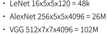
核心思想：

NiN块：卷积层+2 个 11 卷积层， 11 卷积层前后的 ReLU 对每个像素增加了非线性性
模型最后端采用全局平均池化层，来代替 VGG 和 AlexNet 中的全连接层 => 不容易过拟合，更少的参数

 1
 2
 3
 4
 5
 6
 7
 8
 9
10
11
12


import torch
from torch import nn
from d2l import torch as d2l

# 定义：NiN块
def nin_block(in_channels, out_channels, kernel_size, strides, padding):
    return nn.Sequential(
        # 直接代入输入的参数
        nn.Conv2d(in_channels, out_channels, kernel_size, strides, padding),
        nn.ReLU(),
        nn.Conv2d(out_channels, out_channels, kernel_size=1), nn.ReLU(),
        nn.Conv2d(out_channels, out_channels, kernel_size=1), nn.ReLU())

 1
 2
 3
 4
 5
 6
 7
 8
 9
10
11
12
13
14
15
16
17
18
19
20
21
22
23
24
25
26
27
28
29
30
31
32
33
34
35
36


net = nn.Sequential(
    # 灰度图输入通道为1
    nin_block(1, 96, kernel_size=11, strides=4, padding=0),
    nn.MaxPool2d(3, stride=2),
    nin_block(96, 256, kernel_size=5, strides=1, padding=2),
    nn.MaxPool2d(3, stride=2),
    nin_block(256, 384, kernel_size=3, strides=1, padding=1),
    nn.MaxPool2d(3, stride=2),
    nn.Dropout(0.5),
    # 标签类别数是10（Fashion_MNIST）
    nin_block(384, 10, kernel_size=3, strides=1, padding=1),
    # 高宽都变为1
    nn.AdaptiveAvgPool2d((1, 1)),
    # 将四维的输出转成二维的输出，其形状为(批量大小,10)
    nn.Flatten())

# 查看输出形状
X = torch.rand(size=(1, 1, 224, 224))
for layer in net:
    X = layer(X)
    print(layer.__class__.__name__,'output shape:\t', X.shape)
# Sequential output shape:     torch.Size([1, 96, 54, 54])
# MaxPool2d output shape:      torch.Size([1, 96, 26, 26])
# Sequential output shape:     torch.Size([1, 256, 26, 26])
# MaxPool2d output shape:      torch.Size([1, 256, 12, 12])
# Sequential output shape:     torch.Size([1, 384, 12, 12])
# MaxPool2d output shape:      torch.Size([1, 384, 5, 5])
# Dropout output shape:        torch.Size([1, 384, 5, 5])
# Sequential output shape:     torch.Size([1, 10, 5, 5])
# AdaptiveAvgPool2d output shape:      torch.Size([1, 10, 1, 1])
# Flatten output shape:        torch.Size([1, 10])

# 训练
lr, num_epochs, batch_size = 0.1, 10, 128
train_iter, test_iter = d2l.load_data_fashion_mnist(batch_size, resize=224)
d2l.train_ch6(net, train_iter, test_iter, num_epochs, lr, d2l.try_gpu())

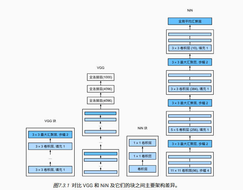
含并行连结的网络 GoogLeNet

Inception 块

输入和输出的宽高相等，但通道数改变
白色快用来改变通道数，蓝色块用来抽取信息
和 33 或 55 卷积层相比，Inception 块的参数个数更少，计算复杂度更低
由后续各种变种 V2、V3、V4

GoogLeNet

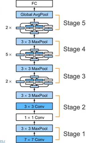
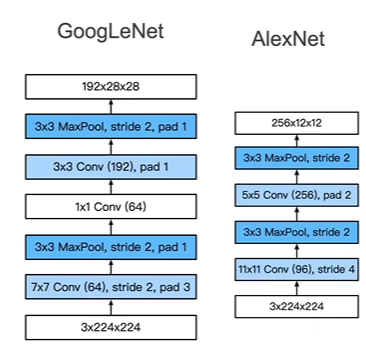
Stage 1 & 2

GoogLeNet 使用了更小的卷积层，最终的宽高更大，从而之后可以使用更深的网络

Stage 3

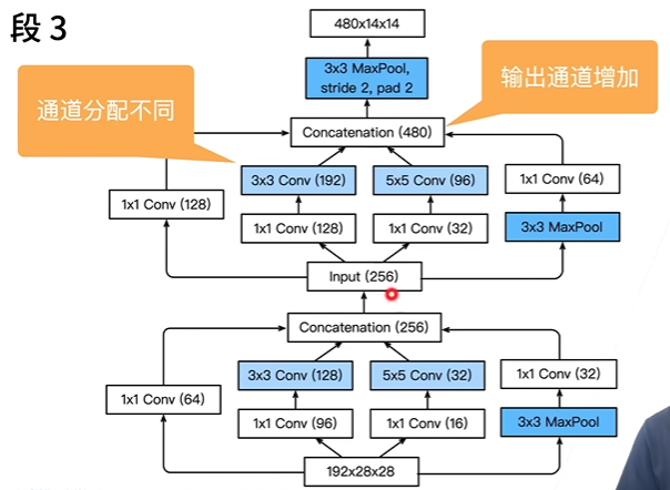
通道分配基本无规律可总结

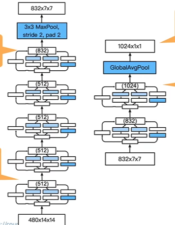
Stage 4 & 5

代码实现

7.4. 含并行连结的网络（GoogLeNet） — 动手学深度学习 2.0.0 documentation

照着网络敲代码

 1
 2
 3
 4
 5
 6
 7
 8
 9
10
11
12
13
14
15
16
17
18
19
20
21
22
23
24
25
26
27
28
29
30
31
32
33
34
35
36
37
38
39
40
41
42
43
44
45
46
47
48
49
50
51
52
53
54
55
56
57
58
59
60
61
62
63
64
65
66
67
68


import torch
from torch import nn
from torch.nn import functional as F
from d2l import torch as d2l


class Inception(nn.Module):
    # c1--c4是每条路径的输出通道数
    def __init__(self, in_channels, c1, c2, c3, c4, **kwargs):
        super(Inception, self).__init__(**kwargs)
        # 线路1，单1x1卷积层
        self.p1_1 = nn.Conv2d(in_channels, c1, kernel_size=1)
        # 线路2，1x1卷积层后接3x3卷积层
        self.p2_1 = nn.Conv2d(in_channels, c2[0], kernel_size=1)
        self.p2_2 = nn.Conv2d(c2[0], c2[1], kernel_size=3, padding=1)
        # 线路3，1x1卷积层后接5x5卷积层
        self.p3_1 = nn.Conv2d(in_channels, c3[0], kernel_size=1)
        self.p3_2 = nn.Conv2d(c3[0], c3[1], kernel_size=5, padding=2)
        # 线路4，3x3最大汇聚层后接1x1卷积层
        self.p4_1 = nn.MaxPool2d(kernel_size=3, stride=1, padding=1)
        self.p4_2 = nn.Conv2d(in_channels, c4, kernel_size=1)

    def forward(self, x):
        p1 = F.relu(self.p1_1(x))
        p2 = F.relu(self.p2_2(F.relu(self.p2_1(x))))
        p3 = F.relu(self.p3_2(F.relu(self.p3_1(x))))
        p4 = F.relu(self.p4_2(self.p4_1(x)))
        # 在通道维度上连结输出
        return torch.cat((p1, p2, p3, p4), dim=1)

b1 = nn.Sequential(nn.Conv2d(1, 64, kernel_size=7, stride=2, padding=3),
                   nn.ReLU(),
                   nn.MaxPool2d(kernel_size=3, stride=2, padding=1))
b2 = nn.Sequential(nn.Conv2d(64, 64, kernel_size=1),
                   nn.ReLU(),
                   nn.Conv2d(64, 192, kernel_size=3, padding=1),
                   nn.ReLU(),
                   nn.MaxPool2d(kernel_size=3, stride=2, padding=1))
b3 = nn.Sequential(Inception(192, 64, (96, 128), (16, 32), 32),
                   Inception(256, 128, (128, 192), (32, 96), 64),
                   nn.MaxPool2d(kernel_size=3, stride=2, padding=1))
b4 = nn.Sequential(Inception(480, 192, (96, 208), (16, 48), 64),
                   Inception(512, 160, (112, 224), (24, 64), 64),
                   Inception(512, 128, (128, 256), (24, 64), 64),
                   Inception(512, 112, (144, 288), (32, 64), 64),
                   Inception(528, 256, (160, 320), (32, 128), 128),
                   nn.MaxPool2d(kernel_size=3, stride=2, padding=1))
b5 = nn.Sequential(Inception(832, 256, (160, 320), (32, 128), 128),
                   Inception(832, 384, (192, 384), (48, 128), 128),
                   nn.AdaptiveAvgPool2d((1,1)),
                   nn.Flatten())

net = nn.Sequential(b1, b2, b3, b4, b5, nn.Linear(1024, 10))

X = torch.rand(size=(1, 1, 96, 96))
for layer in net:
    X = layer(X)
    print(layer.__class__.__name__,'output shape:\t', X.shape)
# Sequential output shape:     torch.Size([1, 64, 24, 24])
# Sequential output shape:     torch.Size([1, 192, 12, 12])
# Sequential output shape:     torch.Size([1, 480, 6, 6])
# Sequential output shape:     torch.Size([1, 832, 3, 3])
# Sequential output shape:     torch.Size([1, 1024])
# Linear output shape:         torch.Size([1, 10])

lr, num_epochs, batch_size = 0.1, 10, 128
train_iter, test_iter = d2l.load_data_fashion_mnist(batch_size, resize=96)
d2l.train_ch6(net, train_iter, test_iter, num_epochs, lr, d2l.try_gpu())

批量归一化

核心思想

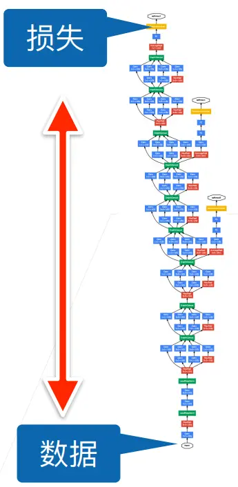
反向传递时，数据由上至下传递。梯度由于相乘，越靠下梯度越小。因此底层的变化会导致上层的数据跟着变，需要重新学习，导致收敛变慢
能否在学习底部的时候尽量避免顶部的变化？
变化是因为每层方差和均值不同，考虑将不同层的不同位置的小批量的分布固定

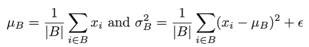（$ \epsilon $确保$ \sigma_B $不为 0）

批量归一化层

作用在全连接层和卷积层的输出上，激活函数前：批量归一化是线性变化
或作用在全连接层和卷积层的输入上
对全连接层的作用是在特征维度上，对卷积层的作用在通道维上
- 特别是 1*1 的卷积核，就是将所有的像素当成样本来计算均值和方差，通道维可以看作是卷积层的特征维

作用

最初想法：减少内部协变量转移（用今天的数据拟合明天）
后续指出：在每个小批量中加入噪音来控制模型复杂度（选取小批量时是随机选取的，因此方差和均值也可看作是随机的）
- 因此没必要和丢弃法 dropout 混合使用

总结：

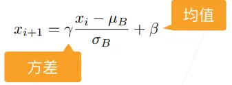
固定小批量中的均值和方差，然后学习出适合的偏移和缩放
可以加快收敛速度，但一般不改变模型精度

代码实现

从零实现

 1
 2
 3
 4
 5
 6
 7
 8
 9
10
11
12
13
14
15
16
17
18
19
20
21
22
23
24
25
26
27
28
29
30
31
32
33
34
35
36
37
38
39
40
41
42
43
44
45
46
47
48
49
50
51
52
53
54
55
56
57
58
59
60
61
62
63
64
65
66
67
68
69
70
71
72
73
74
75


import torch
from torch import nn
from d2l import torch as d2l


def batch_norm(X, gamma, beta, moving_mean, moving_var, eps, momentum):
    # 通过is_grad_enabled来判断当前模式是训练模式还是预测模式
    if not torch.is_grad_enabled():
        # 如果是在预测模式下，直接使用传入的移动平均所得的均值和方差
        X_hat = (X - moving_mean) / torch.sqrt(moving_var + eps)
    else:
        assert len(X.shape) in (2, 4)
        if len(X.shape) == 2:
            # 使用全连接层的情况，计算特征维上的均值和方差
            mean = X.mean(dim=0)
            var = ((X - mean) ** 2).mean(dim=0)
        else:
            # 使用二维卷积层的情况，计算通道维上（axis=1）的均值和方差。
            # 这里我们需要保持X的形状以便后面可以做广播运算
            mean = X.mean(dim=(0, 2, 3), keepdim=True)
            var = ((X - mean) ** 2).mean(dim=(0, 2, 3), keepdim=True)
        # 训练模式下，用当前的均值和方差做标准化
        X_hat = (X - mean) / torch.sqrt(var + eps)
        # 更新移动平均的均值和方差
        moving_mean = momentum * moving_mean + (1.0 - momentum) * mean
        moving_var = momentum * moving_var + (1.0 - momentum) * var
    Y = gamma * X_hat + beta  # 缩放和移位
    return Y, moving_mean.data, moving_var.data

class BatchNorm(nn.Module):
    # num_features：完全连接层的输出数量或卷积层的输出通道数。
    # num_dims：2表示完全连接层，4表示卷积层
    def __init__(self, num_features, num_dims):
        super().__init__()
        if num_dims == 2:
            shape = (1, num_features)
        else:
            shape = (1, num_features, 1, 1)
        # 参与求梯度和迭代的拉伸和偏移参数，分别初始化成1和0
        self.gamma = nn.Parameter(torch.ones(shape))
        self.beta = nn.Parameter(torch.zeros(shape))
        # 非模型参数的变量初始化为0和1
        self.moving_mean = torch.zeros(shape)
        self.moving_var = torch.ones(shape)

    def forward(self, X):
        # 如果X不在内存上，将moving_mean和moving_var
        # 复制到X所在显存上
        if self.moving_mean.device != X.device:
            self.moving_mean = self.moving_mean.to(X.device)
            self.moving_var = self.moving_var.to(X.device)
        # 保存更新过的moving_mean和moving_var
        Y, self.moving_mean, self.moving_var = batch_norm(
            X, self.gamma, self.beta, self.moving_mean,
            self.moving_var, eps=1e-5, momentum=0.9)
        return Y

net = nn.Sequential(
    nn.Conv2d(1, 6, kernel_size=5), BatchNorm(6, num_dims=4), nn.Sigmoid(),
    nn.AvgPool2d(kernel_size=2, stride=2),
    nn.Conv2d(6, 16, kernel_size=5), BatchNorm(16, num_dims=4), nn.Sigmoid(),
    nn.AvgPool2d(kernel_size=2, stride=2), nn.Flatten(),
    nn.Linear(16*4*4, 120), BatchNorm(120, num_dims=2), nn.Sigmoid(),
    nn.Linear(120, 84), BatchNorm(84, num_dims=2), nn.Sigmoid(),
    nn.Linear(84, 10))

lr, num_epochs, batch_size = 1.0, 10, 256
train_iter, test_iter = d2l.load_data_fashion_mnist(batch_size)
d2l.train_ch6(net, train_iter, test_iter, num_epochs, lr, d2l.try_gpu())

net[1].gamma.reshape((-1,)), net[1].beta.reshape((-1,))
# (tensor([0.4863, 2.8573, 2.3190, 4.3188, 3.8588, 1.7942], device='cuda:0',
#         grad_fn=<ReshapeAliasBackward0>),
#  tensor([-0.0124,  1.4839, -1.7753,  2.3564, -3.8801, -2.1589], device='cuda:0',
#         grad_fn=<ReshapeAliasBackward0>))

简洁实现

 1
 2
 3
 4
 5
 6
 7
 8
 9
10


net = nn.Sequential(
    nn.Conv2d(1, 6, kernel_size=5), nn.BatchNorm2d(6), nn.Sigmoid(),
    nn.AvgPool2d(kernel_size=2, stride=2),
    nn.Conv2d(6, 16, kernel_size=5), nn.BatchNorm2d(16), nn.Sigmoid(),
    nn.AvgPool2d(kernel_size=2, stride=2), nn.Flatten(),
    nn.Linear(256, 120), nn.BatchNorm1d(120), nn.Sigmoid(),
    nn.Linear(120, 84), nn.BatchNorm1d(84), nn.Sigmoid(),
    nn.Linear(84, 10))

d2l.train_ch6(net, train_iter, test_iter, num_epochs, lr, d2l.try_gpu())

残差网络 ResNet

由 VGG 更改而来

计算底层梯度时可以直接通过右侧 1*1 卷积层，因此底层也可以得到较大的梯度，这使得 ResNet 可以训练出 1000 层的模型

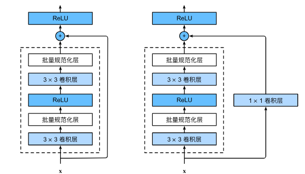
g(x) = f(x) + x

1*1 卷积层调整通道数

 1
 2
 3
 4
 5
 6
 7
 8
 9
10
11
12
13
14
15
16
17
18
19
20
21
22
23
24
25
26
27
28
29
30
31
32
33
34
35
36
37
38
39
40
41
42
43
44
45
46
47
48
49
50
51
52
53


import torch
from torch import nn
from torch.nn import functional as F
from d2l import torch as d2l


class Residual(nn.Module): 
    # use_1x1conv: 是否使用1*1卷积层
    def __init__(self, input_channels, num_channels,
                 use_1x1conv=False, strides=1):
        super().__init__()
        self.conv1 = nn.Conv2d(input_channels, num_channels,
                               kernel_size=3, padding=1, stride=strides)
        self.conv2 = nn.Conv2d(num_channels, num_channels,
                               kernel_size=3, padding=1)
        if use_1x1conv:
            self.conv3 = nn.Conv2d(input_channels, num_channels,
                                   kernel_size=1, stride=strides)
        else:
            self.conv3 = None
        self.bn1 = nn.BatchNorm2d(num_channels)
        self.bn2 = nn.BatchNorm2d(num_channels)

    def forward(self, X):
        Y = F.relu(self.bn1(self.conv1(X)))
        Y = self.bn2(self.conv2(Y))
        if self.conv3:
            X = self.conv3(X)
        Y += X
        return F.relu(Y)

b1 = nn.Sequential(nn.Conv2d(1, 64, kernel_size=7, stride=2, padding=3),
                   nn.BatchNorm2d(64), nn.ReLU(),
                   nn.MaxPool2d(kernel_size=3, stride=2, padding=1))
def resnet_block(input_channels, num_channels, num_residuals,
                 first_block=False):
    blk = []
    # 第一个块特殊处理
    for i in range(num_residuals):
        if i == 0 and not first_block:
            # 通道数加倍，高宽减半
            blk.append(Residual(input_channels, num_channels,
                                use_1x1conv=True, strides=2))
        else:
            blk.append(Residual(num_channels, num_channels))
    return blk
b2 = nn.Sequential(*resnet_block(64, 64, 2, first_block=True))
b3 = nn.Sequential(*resnet_block(64, 128, 2))
b4 = nn.Sequential(*resnet_block(128, 256, 2))
b5 = nn.Sequential(*resnet_block(256, 512, 2))
net = nn.Sequential(b1, b2, b3, b4, b5,
                    nn.AdaptiveAvgPool2d((1,1)),
                    nn.Flatten(), nn.Linear(512, 10))

 1
 2
 3
 4
 5
 6
 7
 8
 9
10
11
12
13
14
15
16


X = torch.rand(size=(1, 1, 224, 224))
for layer in net:
    X = layer(X)
    print(layer.__class__.__name__,'output shape:\t', X.shape)
# Sequential output shape:	 torch.Size([1, 64, 56, 56])
# Sequential output shape:	 torch.Size([1, 64, 56, 56])
# Sequential output shape:	 torch.Size([1, 128, 28, 28])
# Sequential output shape:	 torch.Size([1, 256, 14, 14])
# Sequential output shape:	 torch.Size([1, 512, 7, 7])
# AdaptiveAvgPool2d output shape:	 torch.Size([1, 512, 1, 1])
# Flatten output shape:	 torch.Size([1, 512])
# Linear output shape:	 torch.Size([1, 10])

lr, num_epochs, batch_size = 0.05, 10, 256
train_iter, test_iter = d2l.load_data_fashion_mnist(batch_size, resize=96)
d2l.train_ch6(net, train_iter, test_iter, num_epochs, lr, d2l.try_gpu())