动手学深度学习v2
课程链接:https://courses.d2l.ai/zh-v2/
多层感知机
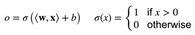
感知机
线性回归:输出实数
Softmax:输出各分类概率
感知机:二分类

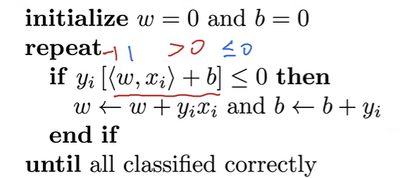
等价于使用批量大小为1的梯度下降
损失函数: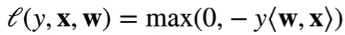
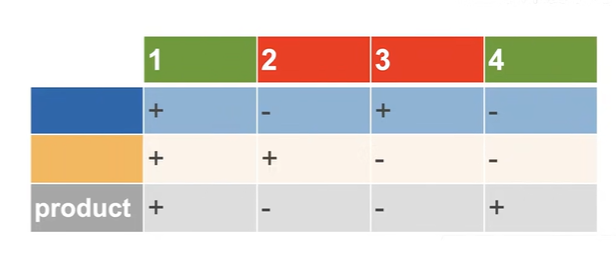
不能拟合XOR函数,只能产生线性分割面
多层感知机
XOR学习
两个分类器进行组合
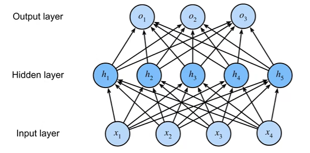
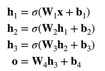
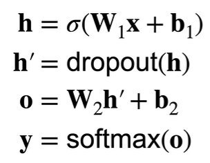
模型
单隐藏层
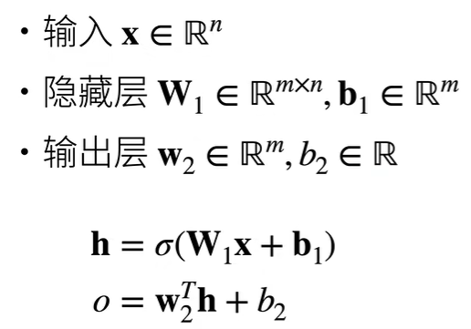
$ \sigma $的加入使得多层感知机不会退化为线性模型
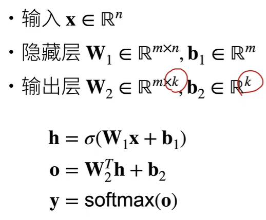
多类分类
通过softmax处理
多隐藏层
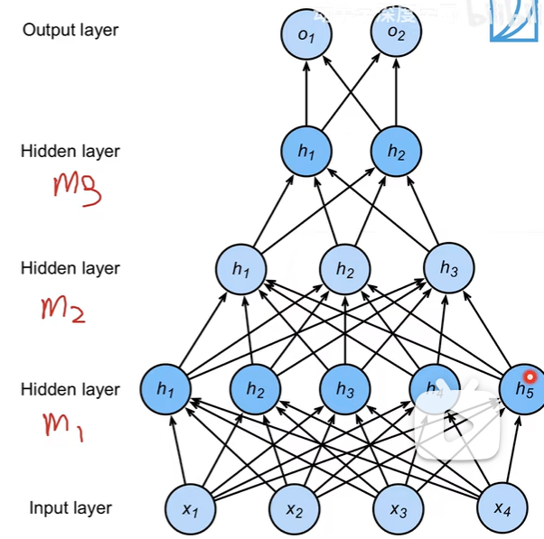
超参数:
- 隐藏层数
- 每层隐藏层大小
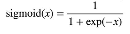
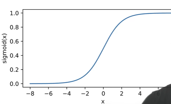
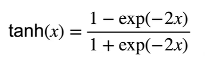
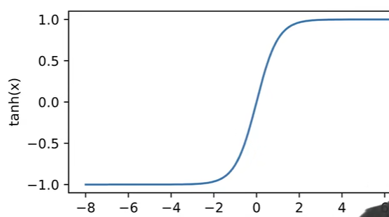
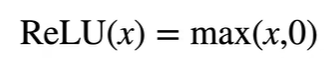
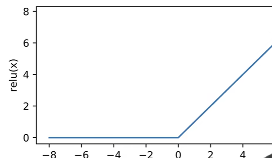
激活函数
代码实现
依旧采用Fashion-MNIST图像分类数据集
手动实现
|
|
简洁实现
|
|
模型选择、欠拟合和过拟合
模型选择
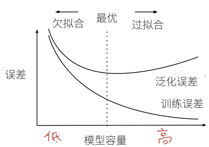
误差
- 训练误差:模型在训练数据上的误差
- 泛化误差:新数据上的误差
我们更关心泛化误差
验证数据集和测试数据集
- 验证数据集:评估模型好坏(不跟训练数据混在一起)
- 测试数据集:只用一次、不可用来调参
K-则交叉验证
没有足够多数据时使用
算法:
- 数据分成K块(K常取5或10)
- for i = 1, …, K,使用第 i 块作为验证数据集,其余用来训练
- 取K个验证集误差的平均
过拟合和欠拟合
| 数据简单 | 数据复杂 | |
|---|---|---|
| 模型容量低 | 正常 | 欠拟合 |
| 模型容量高 | 过拟合 | 正常 |
模型容量
- 模型容量:拟合各种函数的能力
- 低容量:难以拟合训练数据
- 高容量:会记住所有训练数据
- 估计模型容量:
- 不同种类算法间难以比较
- 主要因素:
- 参数个数
- 参数值选择范围
VC维(了解)

深度学习中衡量不准确
权重衰退 weight-decay
使用均方范数作为硬性限制
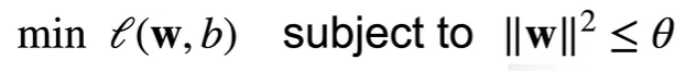
- 限制偏移b没有明显效果
- 较小的$ \theta $意味着更强的正则项
正则项(Regularization term)是机器学习和统计模型中用于防止模型过拟合(overfitting)的一种技术。它通过在损失函数(loss function)中加入一个额外的惩罚项,来约束模型的复杂度,迫使模型在训练时选择较为简单的解,以避免在训练集上表现得过好但在测试集上泛化能力差的问题。
正则项仅在训练过程中使用
使用均方范数作为柔性限制
对任意$ \theta $存在$ \lambda $使得之前的目标函数等于:
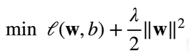
超参数$ \lambda $代表了正则项的重要程度
- $ \lambda = 0 $:无作用
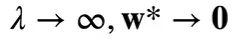
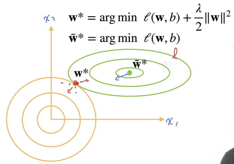
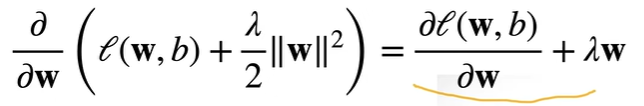
惩罚项的加入使得最优解向原点偏移
- 梯度:
- w随时间t更新:
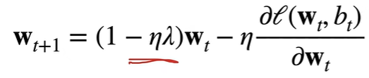
通常衰退$ \eta\lambda < 1 $,因此称作权重衰退
代码实现
从零实现
根据公式生成数据: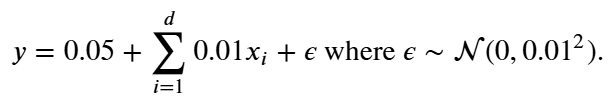
|
|
运行结果:
| $ \lambda $ | 0 | 3 |
|---|---|---|
| w | ||
| loss | 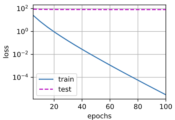 |
 |
简洁实现
|
|
丢弃法 dropout
原理
好的模型需要对输入数据的扰动鲁棒,考虑在层之间加入噪音
无偏差加入噪音:
- 加入噪音前后的期望不变:E[x’] = x
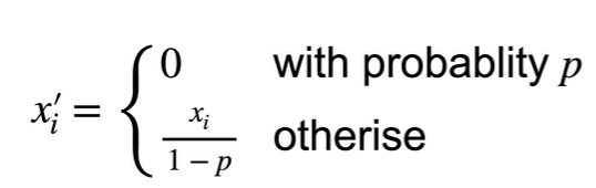 $ x = 0 * p + (1 - p) * x / (1 - p) $
- 丢弃法通常作用在隐藏全连接层的输出上,将一些输出项随机变成0
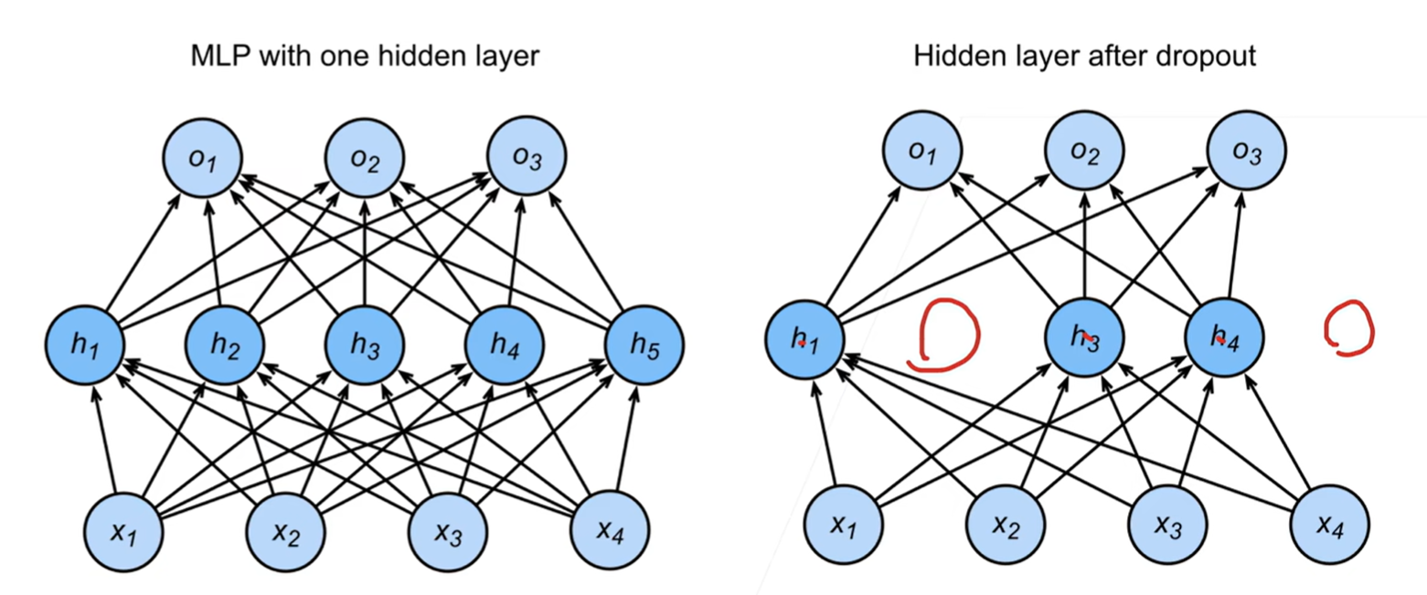
训练:
推理:
推理过程中不使用正则项,丢弃法直接返回输出
h = dropout(h)
代码实现
从零实现
|
|
测试:
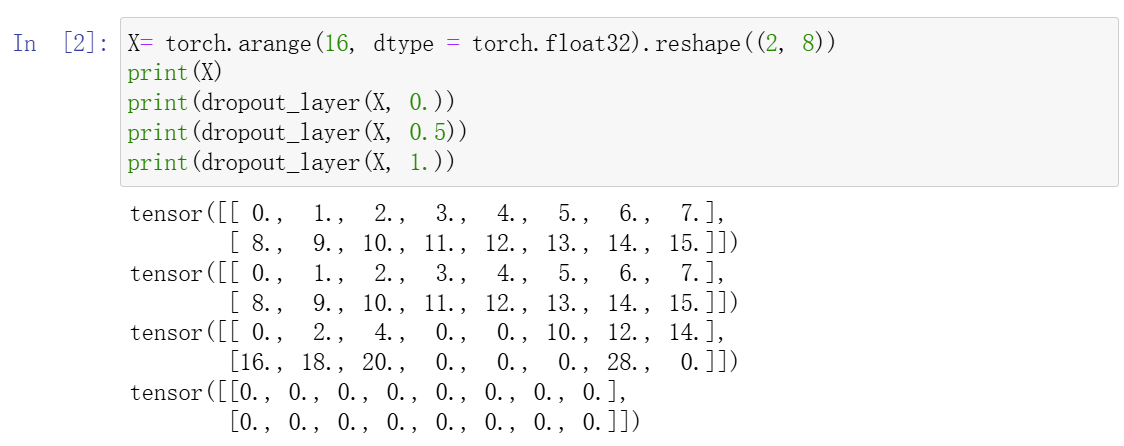
|
|
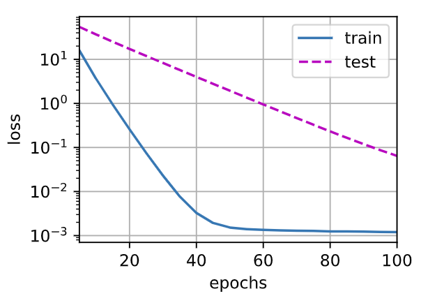
训练结果:
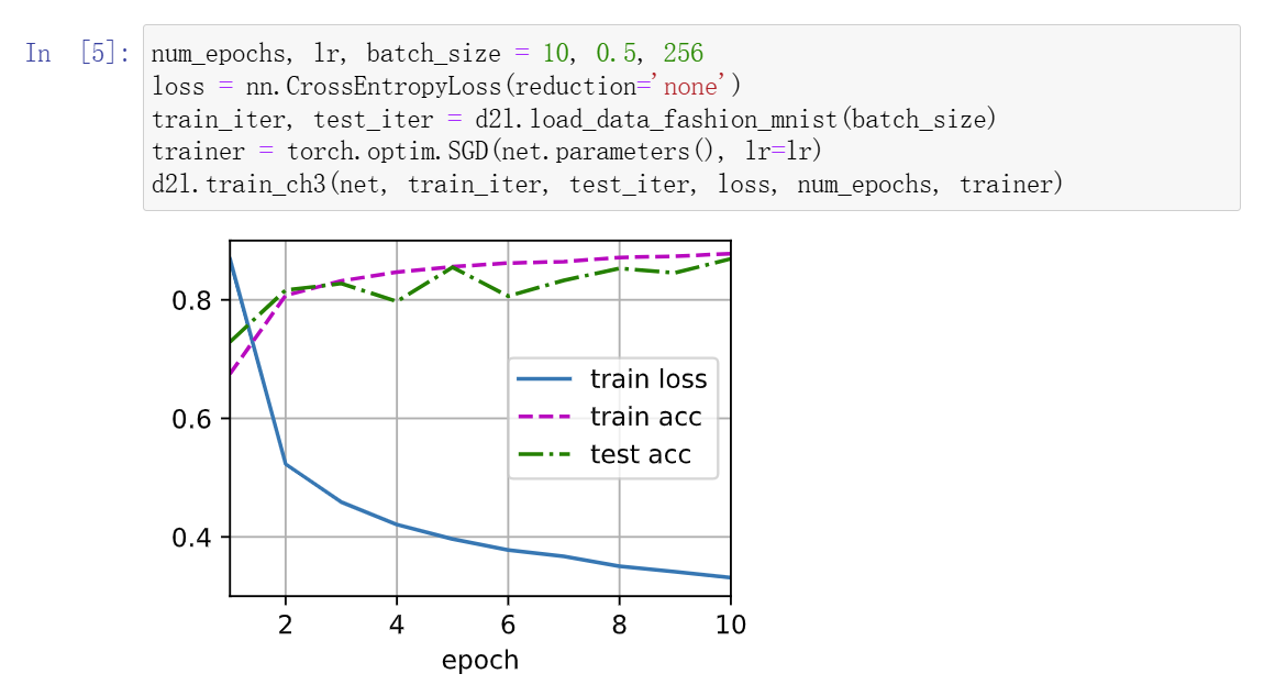
简洁实现
|
|
数值稳定性
考虑一个d层的神经网络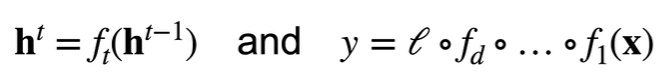
则$ l $关于$ \textbf{W}_t $的梯度为: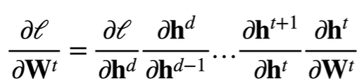
梯度爆炸
例:MLP
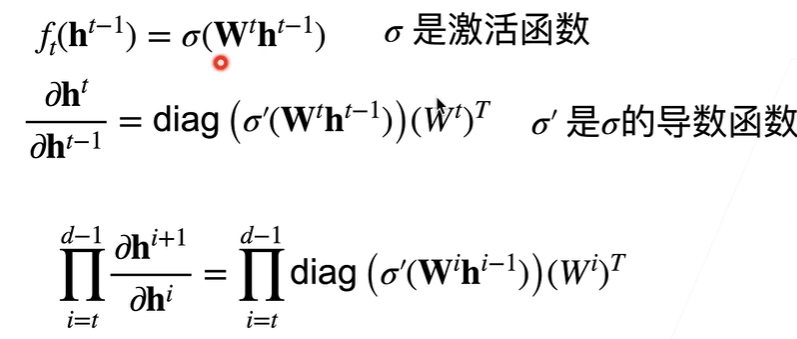
使用ReLU作为激活函数
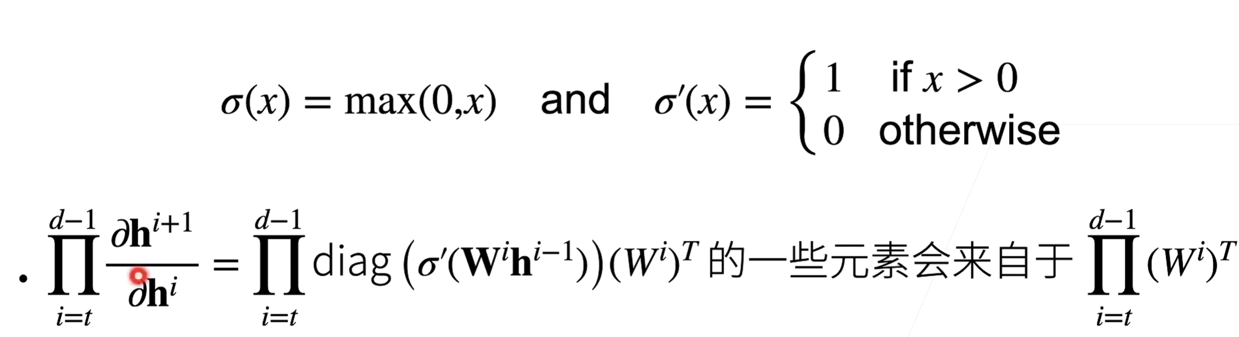
则梯度是Wi中值为1的项做乘法。当d-t较大时,梯度将会非常大
带来问题:
- 值超出值域(对16位浮点数来说尤为严重:6e-5 - 6e4)
- 对学习率敏感
- 过大:梯度更大
- 过小:训练无进展
梯度消失
sigmoid作为激活函数
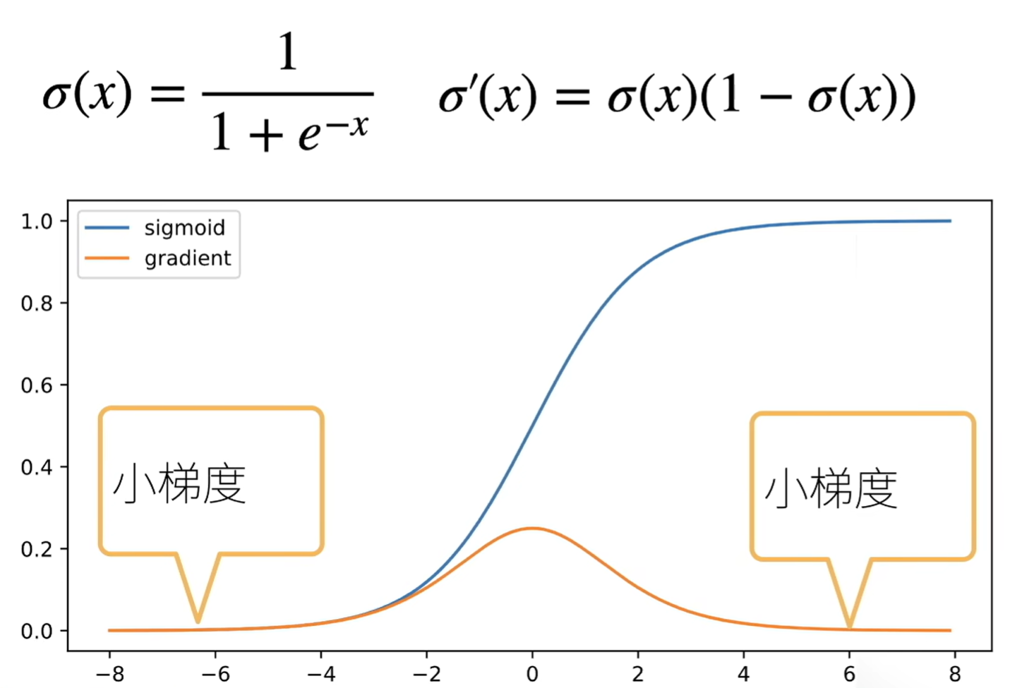
则梯度为d-t个小数值的乘积
带来问题:
- 梯度值变成0
- 无论如何选择学习率,训练无进展
- 限制了神经网络的深度:对较深的神经网络,反向梯度计算使得底层训练效果不好
数值稳定
- 如何让梯度值范围合理?
- 乘法变加法:ResNet、LSTM
- 梯度归一化、梯度剪裁
- 合理的权重初始化和激活函数
我们希望每层的输出和梯度的均值和方差保持一致
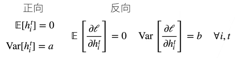
在参数初始化时,最优解附近的表面更加平缓,较远处更容易数值不稳定。因此需要合理的初始化参数
对于正向情况,h与w独立,若使得期望为0,方差为$ \gamma t $,则有$ n{t-1}\gamma_t = 1 $
同样,对于反向情况,有$ n_{t}\gamma_t = 1 $
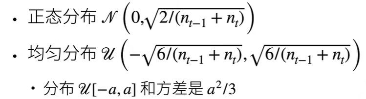
Xavier初始
$ (n_{t-1}\gamma_t + n_{t}\gamma_t)/2 = 1 $
则$ \gamma_t = 2/(n_{t-1}+n_t) $
则参数初始化需满足:
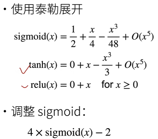
激活函数
假设激活函数为线性
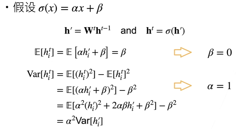
反向的到相同结果,即 f(x) = x
将现有激活函数调整为满足零点附近近似 f(x) = x